Is TabPFN better than XGBoost for credit risk modeling?

On small-to-medium datasets (around 10,000 rows), TabPFN-2.5 outperformed both XGBoost and LightGBM on ROC AUC, PR-AUC, and calibration in a benchmark on Kaggle credit risk data. However, it is 40-100x slower for production credit risk systems.

What is TabPFN and how does it work for tabular data?

TabPFN is a foundation model pre-trained on millions of synthetic tabular datasets. At inference, it takes your training data as context and predicts on new rows using in-context learning, similar to how large language models process text. It requires no hyperparameter tuning.

Can TabPFN be used in production credit risk systems?

Not yet for real-time decisioning. TabPFN's inference latency (5-12 seconds per batch) exceeds production requirements. It also lacks established tooling for regulatory compliance, and model risk management. It is currently best suited for rapid prototyping and challenger model benchmarks.

Can a Foundation Model Replace XGBoost for Credit Risk Modeling?

Are foundation models for tabular data better than gradient boosting for credit risk? The results are clear. Full code and reproducible notebook: Trees vs TabPFN on Colab.

// The AI revolution that skipped tables

We spent years organizing the messy world into clean spreadsheets, just to watch the AI revolution work for the messy world instead.

I build credit risk models. My data lives and dies in a table. And I can tell you firsthand: an enormous share of the work isn’t modeling. It’s turning wildly heterogeneous information into structured features that traditional ML can digest.

So when a foundation model for tables finally showed up, I had to test it where it matters to me: on credit data.

// TabPFN: A Foundation Model for Tabular Data

It was about time. When you train XGBoost (current king of tables), you teach the algorithm to recognize patterns for that specific dataset. The model has never seen another dataset and it starts from zero.

Here comes TabPFN. A Transformer pre-trained on MILLIONS of different synthetic tabular datasets who asks the question: given these training rows AND their labels, what are the best labels for these new rows. Your target variable becomes what LLMs treat as the next token, a simple prediction.

TabPFN removes the need for preprocessing and hyperparameter optimization. — No more preprocessing text, NULLs or hyperparameter optimization.

At inference, TabPFN treats your data as context. The same way an LLM treats the prompt. It processes the whole thing and outputs its predictions. No preprocessing, no feature creation.

// Testing TabPFN on Credit Risk Data

For this experiment, I used Kaggle Credit Risk dataset.

Things I did:

Drop leaky features: no matter how good or frontier your model is, DON’T predict on the future.
Give the trees an advantage: Good hyperparameters, preprocessing. Everything needed to win.

TabPFN just got the data. No help from me:

clf = TabPFNClassifier()
clf.fit(X_train, y_train)

Compare that to the hundreds of lines of preprocessing code for tree-based models, and trees are already the least demanding algorithms when it comes to data preparation.

// Results: TabPFN vs XGBoost vs LightGBM

Each model was trained on the full training set and the holdout was 2,000 samples.

Five-fold cross-validation:

Model	ROC AUC	Std
TabPFN-2.5	0.8728	± 0.0064
LightGBM	0.8466	± 0.0083
XGBoost	0.8377	± 0.0058

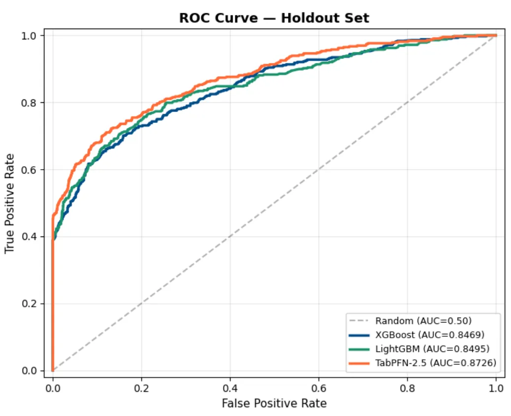
Holdout confirmation:

Model	ROC AUC	PR AUC
TabPFN-2.5	0.8726	0.7738
LightGBM	0.8495	0.7398
XGBoost	0.8469	0.7293

TabPFN won every metric. A 2-3 point AUC gap is significant in credit risk, where models are compared at the third decimal.

ROC curves on holdout set showing TabPFN-2.5 (AUC=0.8726) outperforming LightGBM (0.8495) and XGBoost (0.8469) — ROC curves on the holdout set. TabPFN-2.5 consistently dominates across all operating points.

The cost: TabPFN took 5-12 seconds per fold versus 0.07-0.30 seconds for trees. A 40-100x latency penalty.

// Why Calibration Matters More Than AUC in Credit Risk

Calibration lets the models output actual probabilities (if they’re well calibrated). In Credit Risk, you MUST care because if your model tells you a 15% probability of default you actually want to OBSERVE a 15% of default rate.

AUC is a beauty contest, it tells you the model can rank borrowers. But ranking isn’t enough. Pricing, loss provisioning, capital reserves, regulatory stress testing, all of these depend on the predicted probability of default being accurate, not just ordinally correct.

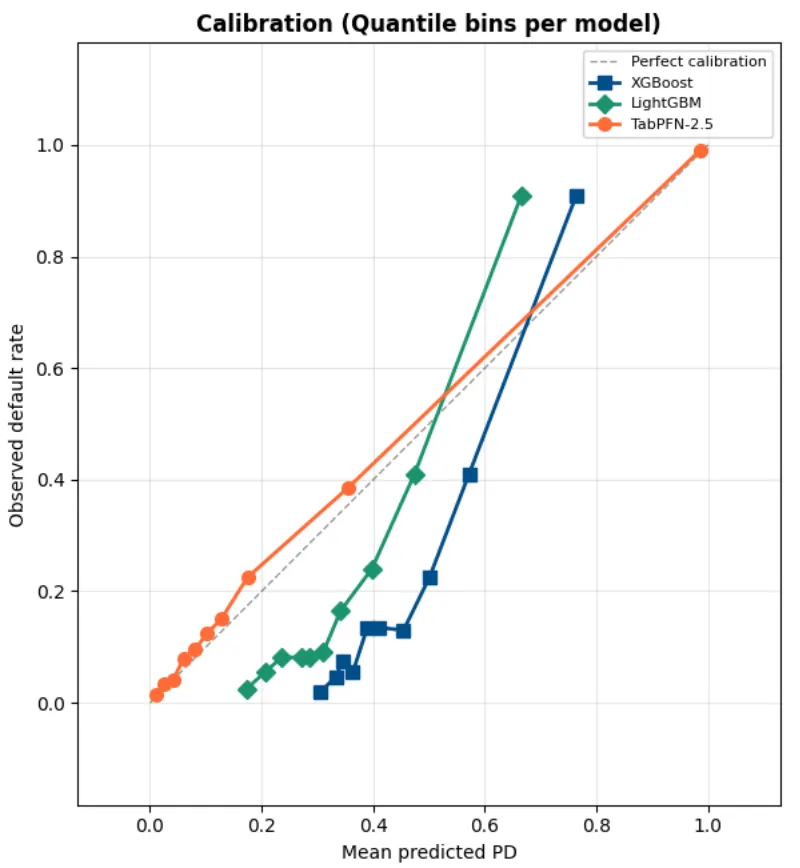
Calibration plot showing TabPFN-2.5 tracking closer to the perfect calibration diagonal than XGBoost and LightGBM — Calibration curves (quantile bins). TabPFN tracks the diagonal of a perfectly calibrated model more closely.

TabPFN delivers calibrated probabilities out of the box. No isotonic regression. No Platt scaling. No post-hoc fix. The probabilities are right because the model is doing Bayesian inference, averaging over possible explanations rather than committing to a single tree structure.

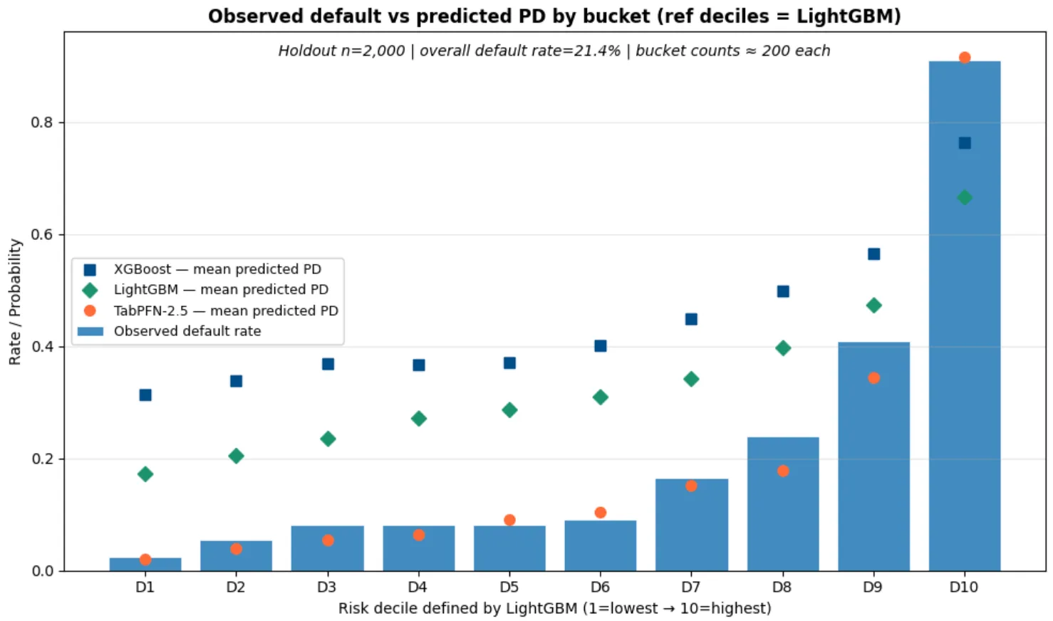
Observed default rate versus predicted probability of default by risk decile, showing TabPFN predictions align more closely with observed rates — Observed default rate vs. predicted PD by risk decile. TabPFN’s predictions align more tightly with actual outcomes across the risk spectrum.

Look at the predictions from the tree-based models. Constantly higher than the observed default rate making the models much more conservative and wildly uncalibrated.

// Where TabPFN Falls Short: Scale, and Latency

Before you replace all of your models, think about this:

Sample size limits: TabPFN-2.5 handles up to ~50,000 samples and 2,000 features. That covers a lot of credit modeling use cases: early-stage fintech, niche portfolios, segments with limited history. But if you’re scoring a 10-million-row mortgage portfolio, you’ll need sampling strategies or a hybrid approach.
Speed: In real-time decisioning at scale, latency matters. Prior Labs is working on a distillation engine that promises tree-level latency with foundation-model accuracy, but it’s not open source yet.

And above all, this was ONE dataset. You should test TabPFN on your data, with your features, against your tuned pipeline.

// What TabPFN Means for Credit Risk Modeling

A foundation model just delivered strong credit risk performance with no domain knowledge, no feature engineering, and no hyperparameter tuning.

It’s not production-ready yet. Sample size limits and latency concerns are real.

Domain expertise is staying for now: translating model outputs into business decisions, satisfying model risk requirements, knowing which features leak; that is staying.